A Guide to Statistics on Historical Trends in Income Inequality
The broad facts of income inequality over the past seven decades are easily summarized:
- The years from the end of World War II into the 1970s were ones of substantial economic growth and broadly shared prosperity.
- Incomes grew rapidly and at roughly the same rate up and down the income ladder, roughly doubling in inflation-adjusted terms between the late 1940s and early 1970s.
- The gap between those high up the income ladder and those on the middle and lower rungs — while substantial — did not change much during this period.
- Beginning in the 1970s, economic growth slowed and the income gap widened.
- Income growth for households in the middle and lower parts of the distribution slowed sharply, while incomes at the top continued to grow strongly.
- The concentration of income at the very top of the distribution rose to levels last seen nearly a century ago, during the “Roaring Twenties.”
- Wealth — the value of a household’s property and financial assets, minus the value of its debts — is much more highly concentrated than income. The best survey data show that the share of wealth held by the top 1 percent rose from 30 percent in 1989 to 39 percent in 2016, while the share held by the bottom 90 percent fell from 33 percent to 23 percent.
Data from a variety of sources contribute to this broad picture of strong growth and shared prosperity for the early postwar period, followed by slower growth and growing inequality since the 1970s. Within these broad trends, however, different data tell slightly different parts of the story, and no single data source is best for all purposes.
This guide consists of four sections. The first describes the commonly used sources and statistics on income and discusses their relative strengths and limitations in understanding trends in income and inequality. The second provides an overview of the trends revealed in those key data sources. The third and fourth sections supply additional information on wealth, which complements the income data as a measure of how the most well-off Americans are doing, and poverty, which measures how the least well-off Americans are doing.
I. The Census Survey and IRS Income Data
The most widely used sources of data and statistics on household income and its distribution are the annual household survey conducted as part of the Census Bureau’s Current Population Survey (CPS) and the Internal Revenue Service’s (IRS) Statistics of Income (SOI) data compiled from a large sample of individual income tax returns. The Census Bureau publishes annual reports on income, poverty, and health insurance coverage in the United States based on the CPS data,[1] and the IRS publishes an annual report on individual income tax returns based on the SOI.[2] While the Federal Reserve also collects income data in its triennial Survey of Consumer Finances (SCF),[3] the SCF is more valuable as the best source of survey data on wealth.
Each agency produces its own tables and statistics and makes a public-use file of the underlying data available to other researchers. In addition, the Congressional Budget Office (CBO) has developed a model that combines CPS and SOI data to estimate household income both before and after taxes, as well as average taxes paid by income group back to 1979.[4] Economists Thomas Piketty and Emmanuel Saez have used SOI data to construct estimates of the concentration of income at the top of the distribution back to 1913.[5] More recently, they and their colleague Gabriel Zucman have expanded that work to examine trends in wealth concentration and to incorporate the portion of national income not captured in the tax or survey data into their analysis of income inequality.[6] CBO and Piketty, Saez, and Zucman regularly release reports incorporating the latest available data.
Concepts of Income Measured in Census and IRS Data
Census Money Income
The Census Bureau bases its report on income and poverty on a sample of about 68,300 interviews[7] conducted through the Annual Social and Economic Supplement (ASEC) to the monthly CPS, which is the primary source of data for estimating the unemployment rate and other household employment statistics.[8] The ASEC, also called the March CPS,[9] provides information about the total annual resources available to families. These include income from earnings, dividends, and cash benefits (such as Social Security), as well as the value of tax credits such as the Earned Income Tax Credit (EITC) and non-cash benefits such as nutritional assistance, Medicare, Medicaid, public housing, and employer-provided fringe benefits.
The income measure featured in the Census report is money income[10] before taxes, and the unit of analysis is the household. The latest data, for 2018, were released in September 2019. The statistics on household income are available back to 1967. Census has statistics on family income back to 1947, but because Census defines a “family” as two or more people living in a household who are related by birth, marriage, or adoption, those statistics exclude people who live alone or with others to whom they are not related.
Census’s standard income statistics do not adjust for the size and composition of households. Two households with $40,000 of income rank at the same place on the distributional ladder, even if one is a couple with two children and one is a single individual. An alternative preferred by many analysts is to make an equivalence adjustment based on household size and composition so that the adjusted income of a single person with a $40,000 income is larger than the adjusted income of a family of four with the same income. Equivalence adjustment accounts for the fact that larger families need more total income but less per capita income than smaller families because they can share resources and take advantage of economies of scale. In recent reports, Census has supplemented its measures of income inequality based on household money income with estimates based on equivalence-adjusted income.[11]
For reasons having to do with small sample size, data reporting and processing restrictions, and confidentiality considerations, Census provides more limited information about incomes at the very top of the income distribution than elsewhere in the distribution. For example, Census does not collect information about earnings over $1,099,999 for any given job; earnings above that level are recorded in Census data as $1,099,999.[12]
Income Tax Data
The income tax data used in distributional analysis come from a large sample of tax returns compiled by the IRS’s Statistics of Income Division. For 2017, the sample consisted of about 352,000 returns selected from the roughly 154 million returns filed that year.[13] For the population that files tax returns and for the categories of income that get reported, these administrative data are generally more accurate and more complete than survey data; the CPS, for example, is prone to underreporting of some kinds of income.
However, not all people are required to file tax returns, and tax returns do not reflect all sources of income. Since those not required to file returns likely have limited incomes, tax data do not provide a representative view of low-income households. (This is the mirror image of the CPS’s inadequate coverage of high-income households.) Like Census money income, income reported on tax returns excludes non-cash benefits such as SNAP (formerly known as food stamps), housing subsidies, Medicare, Medicaid, and non-taxable employer-provided fringe benefits.
The exclusion of non-filers is a major limitation of the tax data for distributional analysis. A further complication is that the data are available only for “tax-filing units,” not by household or family. (Members of the same family or household may file separate tax returns.)
SOI tax data are also less timely than Census data. Final statistics for tax year 2017 were released in late 2019.
Key Historical Series Constructed From Census and IRS Data
CBO’s Distribution of Household Income
CBO produces annual estimates of the distribution of household income and taxes that combine information from the CPS and the SOI.[14] Thus, these estimates have relatively detailed information about very high-income households and taxes paid (the strengths of the SOI) and about low-income households’ income and non-cash benefits (the strengths of the CPS). CBO also uses expanded measures of household income that include more sources of income than either CPS- or SOI-based measures alone.
Over the years, CBO has made some significant changes to its methodology for analyzing the distribution of income and taxes, notably to how it values government-provided health insurance, which income measure it uses to rank households in analyzing the effects of transfers (government payments) and taxes on inequality, and how it adjusts for inflation (see the Appendix for more detail).
In recent reports CBO employs three income measures:
- Market income, which consists of labor income (wages and fringe benefits), business income, capital income (dividends, interest, and capital gains), income received in retirement for past services (e.g., private pensions), and other non-governmental income sources;
- Income before transfers and taxes, which consists of market income plus social insurance benefits (including Social Security, Medicare, unemployment insurance, and workers’ compensation); and
- Income after transfers and taxes, which consists of income before transfers and taxes plus means-tested transfers (cash payments and in-kind services provided through federal, state, and local government assistance programs to people with relatively low incomes or few assets) minus federal individual and corporate income taxes, payroll taxes, and excise taxes. The largest sources of means-tested transfers are Medicaid and the Children’s Health Insurance Program, SNAP, and Supplemental Security Income.)
CBO uses income before transfers and taxes to rank households. It adjusts for household size by dividing the household’s income by the square root of the number of people in the household. Thus, the adjusted household income of a single person with $20,000 of income is equivalent to that of a household of four with $40,000.
CBO constructs its distributional tables by ranking individuals by their adjusted household income before transfers and taxes and dividing that ranking into five income groups (quintiles), each containing roughly an equal number of people (with further disaggregation of the top quintile).[15] The quintiles contain slightly different numbers of households, depending on the average household size at different points in the income distribution.
One difficult issue in using an expanded definition of income, as CBO does, is how to treat government-provided health insurance such as Medicare and Medicaid. While it has not always done so, CBO now treats the average cost to the government of providing health insurance to eligible households as household income. It essentially does the same for employer-provided health insurance. While government-provided health insurance certainly increases a household’s well-being, it is not the same as money income or near-cash transfers like SNAP benefits because it does not directly help households of limited means meet basic needs such as food, clothing, and shelter.[16] Moreover, part of the government’s cost reflects administrative costs and health industry profits. Since medical benefits make up a sizeable and growing share of income in CBO’s series, this treatment of government-provided health insurance as equivalent to cash income can create differences between trends in CBO’s income data, which include these benefits, and trends in other income series that do not include these benefits, as discussed in Part II.
The latest CBO report on the distribution of household income, released in July 2019, includes data for 1979-2016 on income before and after transfers and taxes as well as taxes paid for each quintile and for the top 1, 5, and 10 percent of households. Because of the effort involved in preparing these analyses, CBO’s annual updates tend to lag behind other sources of income data, often by a couple of years.
Piketty-Saez Data on Income Concentration
Economists Thomas Piketty and Emmanuel Saez first published income inequality statistics in 2003 based on IRS data back to 1913 to provide a long-term perspective on trends in income concentration within the top 10 percent of the distribution.[17] They focused on the top of the income distribution because prior to World War II, only about 10 to 15 percent of potential tax units had to file an income tax return.
Their income concept is market income before individual income taxes. They define market income as the sum of all income sources reported on tax returns, including realized capital gains[18] and taxable unemployment compensation.[19] Other non-taxable non-cash income sources, such as nutrition assistance and employer-provided health care benefits, are not included.
People with market income who are not required to file income tax returns do not show up in the population of tax filers, and their income does not show up in the total income reported on tax returns.[20] Piketty and Saez address these omissions by estimating the number of non-filers and their income and adding these to the population of tax filers and the market income calculated from the income tax data.[21] They compute total income as all market income reported on tax returns plus their estimate of market income for non-filers.[22] The top 10 percent, top 1 percent, etc. are defined with respect to this total income and to the population of potential tax units (filers plus non-filers). Piketty and Saez do not make an adjustment for family size in their analysis.
The primary advantage of these Piketty-Saez data is that they provide the longest historical series of annual data on income at the top of the distribution. The key limitation is that they are based exclusively on tax return data. As a result, they do not include data for individual non-filers (and therefore provide no information about the distribution of income among non-filers). Nor do they account for government cash transfers or public and private non-cash benefits.
These public and private non-cash benefits, which are missing from the Piketty-Saez income measure, constitute a growing share of personal income.[23] As a result, the Piketty-Saez measure captures a declining share of personal income in the national income and product accounts over time, possibly distorting estimates of the share of total income growth occurring at the top of the distribution.[24]
Recent work by Piketty, Saez, and Zucman tries to address this concern by ambitiously combining tax, survey, and national accounts data to estimate the distribution of total national income, both before and after transfers and taxes.[25] They allocate all national income to U.S. residents age 20 or older, with married couples’ income split equally in their base case.[26] As the authors acknowledge, however, “imputing all national income, taxes, transfers, and public goods spending requires making assumptions on a number of complex issues, such as the economic incidence of taxes and who benefits from government spending.”[27]
II. Broad Trends in Income Inequality
Because each individual source of readily available data on income distribution has different advantages and limitations, no single source illustrates all of the major trends in inequality over the past six decades or so. Ideally, we would look at a comprehensive measure of income that covers a long time span, allows us to compare income before and after transfers and taxes at different points in the distribution, and accounts for changes in household size and composition.
CBO data satisfy many of these criteria but only go back to 1979 and are sensitive to particular methodological choices. (See the Appendix.) The historical Census family income data series and Piketty-Saez top-income concentration data cover a longer time span but use less comprehensive income measures and do not adjust for changes in household size and composition. Using a more comprehensive income measure, as Piketty, Saez, and Zucman do in their statistics on the distribution of national income, addresses some issues but raises others because of the number of assumptions involved.
The Loss of Shared Prosperity
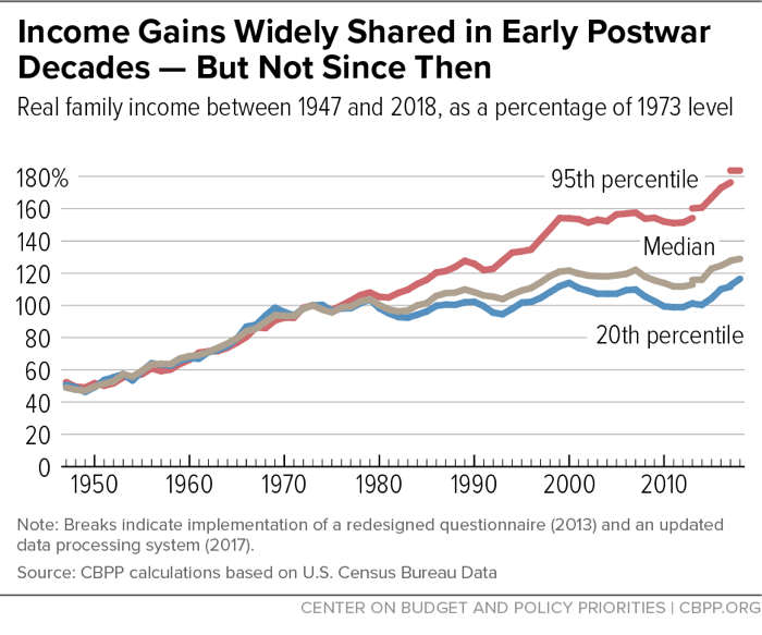
Census family income data show that from the late 1940s to the early 1970s, incomes across the distribution grew at nearly the same pace. Figure 1 shows the level of real (inflation-adjusted) income at several points on the distribution relative to its 1973 level. [28] It shows that real family income roughly doubled from the late 1940s to the early 1970s at the 95th percentile (the income level separating the highest-income 5 percent of families from the remaining 95 percent), at the median (the income level separating the upper half of families from the lower half), and at the 20th percentile (the income level separating the bottom fifth of families from the remaining four-fifths).
Then, beginning in the 1970s, income disparities began to widen, with income growing much faster at the top of the ladder than in the middle or bottom. Household (as opposed to family) income data, which are available only since 1967, show a similar pattern of widening inequality and scant growth in median income and income at the 20th percentile following the 1999 and 2007 business cycle peaks.
While the Census family income data are useful for illustrating that income inequality began widening in the 1970s, other data are superior for assessing more recent trends.
Widening Inequality Since the 1970s
Census family income data show that the era of shared prosperity ended in the 1970s and illustrate the divergence in income since then. CBO data allow us to look at what has happened to comprehensive income measures since 1979 — both before and after transfers and taxes — and offer a better view of what has happened at the top of the distribution.
As Figure 2 shows, from 1979 to 2007 (just before the financial crisis and Great Recession), average income after transfers and taxes quadrupled for the top 1 percent of the distribution.[29] The increases were much smaller for the middle 60 percent and bottom 20 percent of the distribution.
The CBO data also show income growth for the bottom 20 percent over this period that’s comparable to the 81st through 99th percentiles and substantially greater than the middle 60 percent. But this appears to be a methodological anomaly associated with CBO’s 2012 change in how it values government-provided health insurance and its 2018 change in the income measure used to rank households, as described in the Appendix. Together, these changes appear to strongly affect income trends for the poorest households, substantially raising the level and rate of growth of their measured income and perhaps substantially exaggerating the rise in low-income households’ true standard of living.
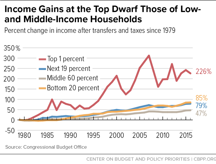
After-tax incomes fell sharply at the top of the distribution in 2008 and 2009 but have since partially recovered. The up-and-down pattern in 2012-13 may reflect, in part, decisions by wealthy taxpayers to sell appreciated assets in 2012 in order to pay taxes on those capital gains before income tax rates increased in 2013. The Piketty-Saez data discussed below, which go through 2018, show a generally upward trend since 2009 that is consistent with this explanation.
Although the average income after transfers and taxes of the top 1 percent of households remains well below its 2007 peak, the percentage increase in their average income after transfers and taxes from 1979 to 2016 was nearly five times that of the middle 60 percent and more than two-and-a-halftimes that of the bottom fifth. (See Table 1.) Moreover, CBO projects that the top 1 percent’s income after transfers and taxes will grow significantly faster than other income groups’ between 2016 and 2021, boosting its cumulative 1979-2021 growth to 281 percent.[30] This suggests that the Great Recession and financial crisis — like the dot-com collapse of the early 2000s — may have had only a temporary impact on the trend of faster income growth at the top.
| TABLE 1 | ||||
|---|---|---|---|---|
| Growth in CBO Comprehensive Income by Income Group and Time Period | ||||
| Growth in average income |
Bottom 20 percent |
Middle 60 percent |
Next 19 percent |
Top 1 percent |
| 1979-2007 | ||||
| Before transfers and taxes | 40% | 31% | 66% | 273% |
| After transfers and taxes | 61% | 41% | 72% | 312% |
| 1979-2016 | ||||
| Before transfers and taxes | 33% | 33% | 75% | 218% |
| After transfers and taxes | 85% | 47% | 79% | 226% |
Trends in income before transfers and taxes look very similar. Because average tax rates have fallen for all income groups since 1979, income before transfers and taxes grew somewhat more slowly than income after transfers and taxes from 1979 to 2016. (See the box for more on the effect of transfers and taxes on income.)
Transfers and Taxes Are Progressive,
But Income Is Highly Concentrated Both Before and After Transfers and Taxes
The charts below, using CBO data, show that the effect of transfers and taxes is progressive: the top 20 percent of households had a smaller share of total income in 2016 after transfers and taxes than before transfers and taxes, while the opposite is true for the other 80 percent of households. (Transfers include state and local government payments, but taxes do not include state and local taxes.)
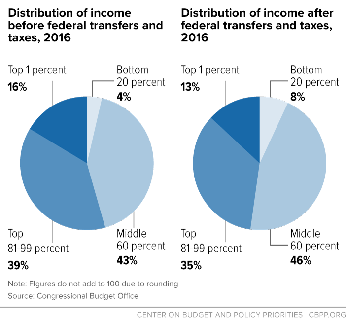
Income is highly concentrated under either measure, however. The top 1 percent of households received 16 percent of income before transfers and taxes and 13 percent of income after transfers and taxes in 2016 — many times their share of the population. The comparable figures for the bottom 80 percent of households were 47 and 54 percent, respectively.
As CBO’s latest analysis of trends in income distribution from 1979 to 2016 shows, both federal transfers and federal taxes reduce income inequality, but the reduction due to transfers is considerably larger.
Income Concentration Has Returned to 1920s Levels
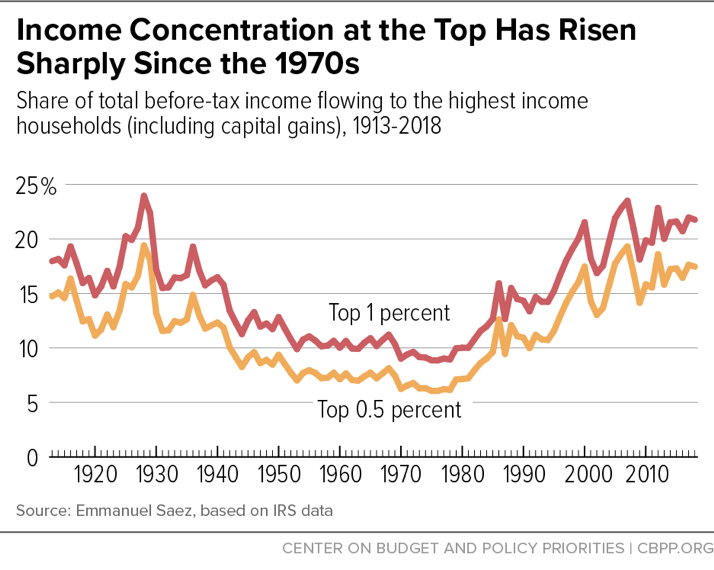
The Piketty-Saez estimates derived from IRS tax data put the increasing concentration of income at the top of the distribution into a longer-term historical context.[31] As Figure 3 shows, the top 1 percent’s share of income before transfers and taxes has been rising since the late 1970s, and in recent decades has climbed to levels not seen since the 1920s. The vast majority of the increase occurred among the top 0.5 percent of households.[32]
The increase in income concentration since the 1970s reversed the prior, long-term downward trend. After peaking in 1928, the share of income held by households at the very top of the income ladder declined through the 1930s and 1940s. Consistent with the shared prosperity found in the Census data on average family income, the share of income received by those at the very top changed little over the 1950s, 1960s, and early 1970s. The sharp rise in income concentration at the top since the late 1970s was interrupted briefly by the dot-com collapse in the early 2000s and again in 2008 with the onset of the financial crisis and Great Recession, but top incomes generally have been on the rise since 2009. The Piketty-Saez data show the same pattern in 2012-16 as CBO’s, with a further rise in top income shares in 2017.
III. The Distribution of Wealth
A family’s income is the flow of money coming in over the course of a year. Its wealth (sometimes referred to as “net worth”) is the total stock of assets it has as a result of inheritance and saving, less any liabilities.[33] Wealth is much more highly concentrated than income, and concentration at the top has risen since the 1980s.
The main official source of data for the distribution of household wealth is the Federal Reserve’s Survey of Consumer Finances (SCF), conducted every three years. SCF data go back to 1983; the latest published data are for 2016. The SCF is based on a sample of about 6,300 families. The data sources discussed in the preceding sections on income distribution are superior to the SCF for measuring income distribution, but none of those sources has comparable data for looking at the distribution of wealth.
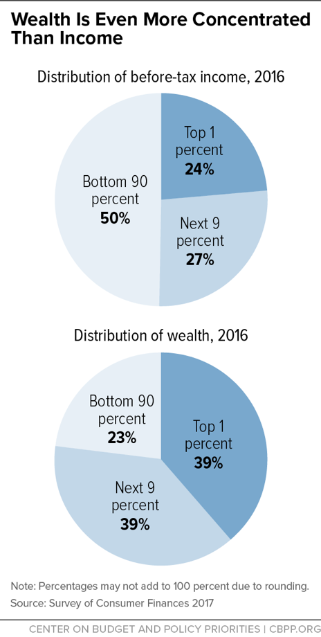
The latest SCF, for 2016, provides detailed statistics on wealth and income showing that wealth is much more concentrated than income.[34] (See Figure 4.) It should be noted that while there is considerable overlap, the top 1 percent of the income distribution does not contain exactly the same people as the top 1 percent of the wealth distribution. The SCF data show that the top 1 percent of the income distribution received roughly a quarter of all income in 2016, while the top 1 percent of the wealth distribution held nearly two-fifths of all wealth. Similarly, the top 10 percent of the income distribution received a little more than half of all income, while the top 10 percent of the wealth distribution held more than three-quarters of all wealth.
SCF data show that the share of wealth held by the top 1 percent rose from just under 30 percent in 1989 to 38.6 percent in 2016, while the share held by the bottom 90 percent fell from 33.2 percent to 22.8 percent.[35]
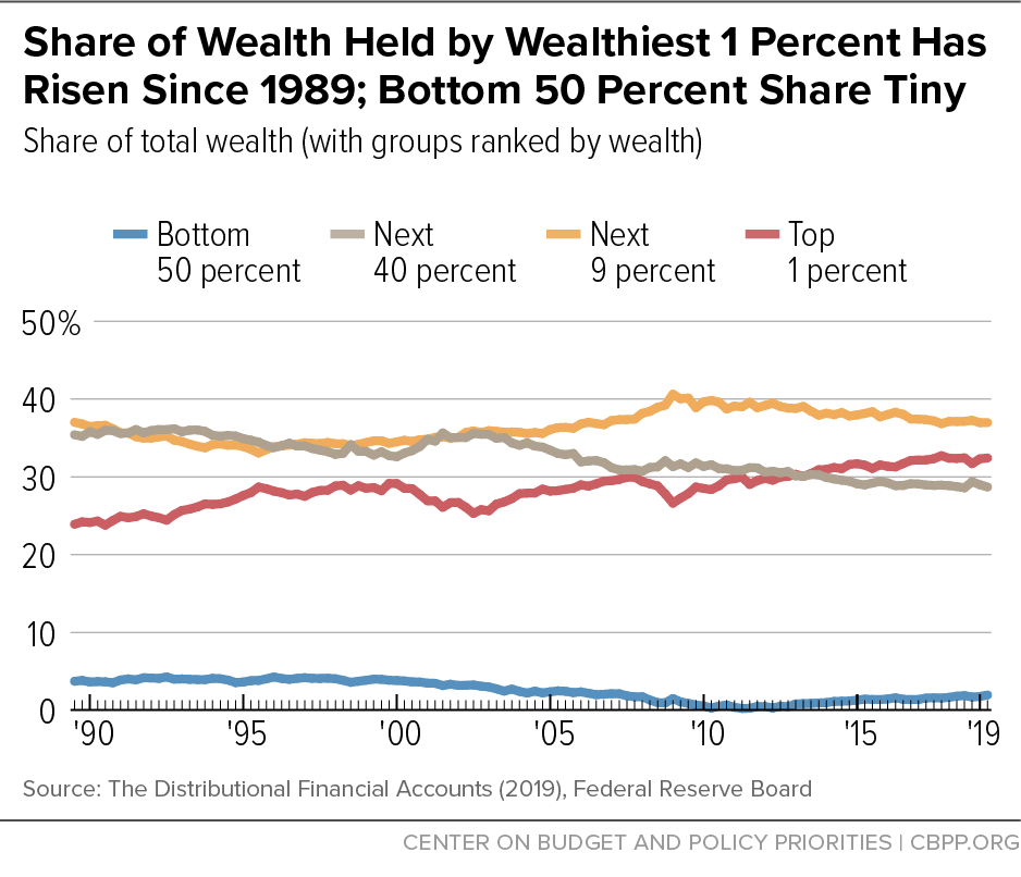
The Fed recently introduced distributional financial accounts that integrate the SCF’s rich distributional information with quarterly data on aggregate balance sheets of major sectors of the U.S. economy from the Fed’s Financial Accounts of the United States.[36] Distributional financial account data begin in 1989, are updated quarterly, and show the share of wealth held by the bottom 50 percent, next 40 percent, next 9 percent, and top 1 percent.
The distributional financial accounts illustrate how little wealth the bottom 50 percent of households have (less than 2 percent) and how much the top 10 percent have (almost three-quarters). They also show that concentration has increased at the top of the wealth distribution since 1989.[37] (See Figure 5.)
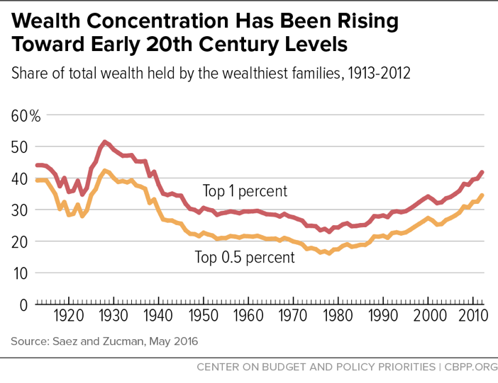
While the Fed data are invaluable, they cover a relatively short period of time. Recently, Emmanuel Saez and Gabriel Zucman have used tax-return information on income derived from wealth to infer the underlying distribution of wealth over time.[38] Figure 6 shows Saez and Zucman’s estimates of the share of wealth held by the top 1 percent and top 0.5 percent since 1913. As with income, these data show a long decline in wealth concentration from the late 1920s into the late 1970s but a marked increase since then, driven by a rising share of wealth at the very top (the top 0.5 percent).[39]
IV. Poverty
The Official Poverty Measure
The official U.S. poverty measure was developed in the 1960s. The Census Bureau uses money income (as described above) to determine a person’s poverty status. Each family or unrelated individual in the population is assigned a money income threshold based on the size of their family and age of its members.[40] A person is defined as living in poverty if their family income is below the threshold for that family size and composition (the threshold for a couple with two children was about $25,500 in 2018). The poverty thresholds are adjusted each year to reflect changes in the consumer price index. The poverty rate is the percentage of people living in poverty.
The official poverty statistics show a sharp decline in the poverty rate between 1959 and 1969 but little real change since then, apart from fluctuations due to the business cycle. For a number of reasons, however, the official measure is an unreliable guide to trends in poverty since 1970 and significantly understates progress in reducing poverty since then. It is based on Census money income, which includes cash assistance but does not count non-cash assistance like SNAP and rental vouchers. It also omits the impact of the tax system, including tax credits for working families like the EITC and Child Tax Credit.
Alternatives to the Official Poverty Measure
Over the years, researchers have raised a number of serious conceptual and measurement concerns about how the official poverty rate is calculated. Following the publication of an important National Academy of Sciences (NAS) report on poverty measurement in 1995,[41] the Census Bureau and the Bureau of Labor Statistics (BLS) explored a number of experimental measures reflecting NAS recommendations. NAS-based measures use a more complete definition of income that includes non-cash benefits and tax credits while subtracting taxes and certain expenses. The NAS also recommended using a modernized poverty line that varies with local housing costs.[42]
Census, with support from BLS, unveiled the newest refinement of the NAS-based measures, called the Supplemental Poverty Measure (SPM), in 2011. This measure reflects recommendations from a federal interagency technical working group that drew on the NAS report and subsequent research. The Census SPM is available from 2009 to 2018.[43] Unlike the official measure, which counts only a family’s cash income, the SPM counts non-cash benefits (SNAP, housing assistance, WIC,[44] school lunch, and home energy assistance) and tax credits (the EITC and Child Tax Credit) as income and subtracts various expenses, namely federal and state income and payroll taxes, child care and other work expenses, out-of-pocket medical expenditures, and child support paid. In addition, it updates the poverty line each year based on Americans’ shifting patterns of spending on basic needs, and it varies the poverty line based on local housing costs and the family’s type of housing (such as renters versus owners with a mortgage). Unmarried partners are counted in the same SPM family, unlike in the official poverty measure and most previous implementations of the NAS measure.
Long-Term Poverty Trends
Since non-cash and tax-based benefits constitute a much larger part of government assistance than 50 years ago, the official poverty measure’s exclusion of these benefits masks progress in reducing poverty. Trying to compare poverty in the 1960s to poverty today using the official measure yields misleading results; it implies that programs like SNAP, the EITC, and rental vouchers — all of which were either small in the 1960s or didn’t yet exist — have no effect in reducing poverty, which clearly is not the case.
While the federal government has only calculated the SPM back to 2009, Columbia University researchers have estimated the SPM back to 1967.[45] Using Census Bureau SPM data starting in 2009 and Columbia SPM data for earlier years, we find that government economic security programs are responsible for a decline in the poverty rate from 26.0 percent in 1967 to 14.4 percent in 2017, based on an “anchored” version of the SPM that uses a poverty line tied to what American families spent on basic necessities in 2018 adjusted back for inflation.[46] (See Figure 7.) Without government assistance, poverty would have been about the same in 2017 as in 1967 under this measure, which indicates the strong and growing role of anti-poverty policies.
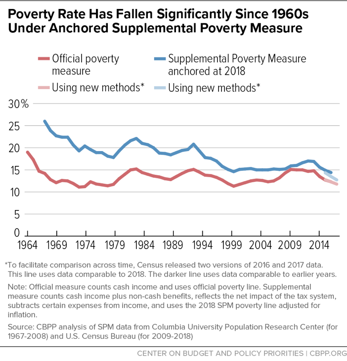
In 2018 poverty fell again, to a record low of 12.8 percent. Data for 2018 are not strictly comparable to those for 1967 due to changes in the Census Bureau’s survey methods,[47] but the Census Bureau provides enough data about this survey transition to make clear that the SPM poverty rate reached a record low in 2018 when using the 2018 SPM poverty line adjusted back for inflation.[48]
Similarly, child poverty reached a record-low 13.7 percent in 2018. Child poverty fell by nearly half over the last 50 years, according to data comparable back to 1967. This improvement is largely due to the growing effectiveness of government assistance policies. Nearly 8 million more children would have been poor in 2018 if the anti-poverty effectiveness of economic security programs (i.e., the safety net of government assistance policies) had remained at its 1967 level.[49] These findings underscore the importance of using the SPM rather than the official poverty measure when evaluating long-term trends in poverty.
Effectiveness of Economic Security Programs Against Poverty
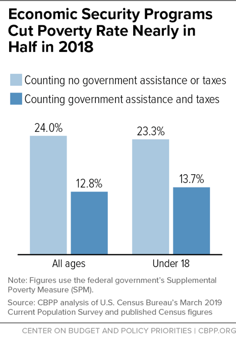
Economic security programs cut poverty nearly in half in 2018, reducing the poverty rate from 24.0 percent to 12.8 percent and lifting 37 million people, including 7 million children, above the poverty line, according to CBPP’s analysis of SPM data.[50] (See Figure 8.)
Further evidence of the effectiveness of these programs is the fact that poverty rose much less in the Great Recession when measured by the SPM rather than the official rate. Between 2007 (the year before the recession) and 2010 (the year after the recession), the anchored SPM rose by 0.7 percentage points, compared to 2.6 percentage points under the official poverty measure. The smaller increase under the SPM largely reflects the wider range of economic security programs included in the SPM and their success in keeping more Americans from falling into poverty during the recession, including the effects of temporary expansions in some economic security programs enacted as part of the 2009 Recovery Act.
Deep Poverty
Measuring “deep” poverty, often defined as income below half of the poverty line, poses particular challenges due to underreporting of certain benefits, reflecting respondents’ forgetfulness, embarrassment about receiving benefits, or other reasons. Census’s counts of program participants typically fall well short of the totals shown in actual administrative records. Such underreporting is common in household surveys and can affect estimates of poverty and, in particular, deep poverty because people who underreport their benefits naturally make up a larger share of those with the lowest reported incomes. (While respondents may also underreport earned income, the net rate of underreporting in the CPS is thought to be much lower for earnings than for benefits.)
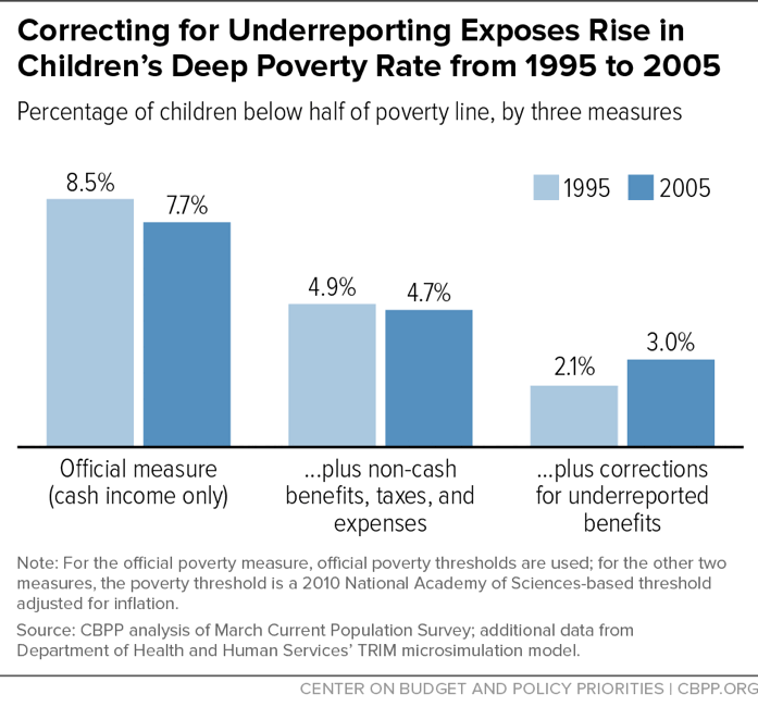
In an analysis that corrects for underreporting of Temporary Assistance for Needy Families (TANF), SNAP, and Supplemental Security Income benefits and uses a comprehensive NAS-based poverty measure similar to the SPM, CBPP analysts find that starting in the mid-1990s — when policymakers made major changes in the public assistance system — the share of children living in poverty fell but the share living in deep poverty rose,[51] from 2.1 percent in 1995 to 3.0 percent in 2005.[52]
Notably, uncorrected CPS figures — whether using the official poverty definition or CBPP’s broader NAS measure — do not show this rise in deep child poverty. By the official measure, the share of children below half the poverty line fell from 1995 to 2005, from 8.5 percent to 7.7 percent. When counting non-cash benefits and taxes but not correcting for underreporting, the figures are essentially flat, at 4.9 percent in 1995 and 4.7 percent in 2005. Only the corrected figures show the increase. (See Figure 9.)
The increase in deep poverty for children was largely due to means-tested cash assistance benefits becoming less effective at shielding children from deep poverty. Over the 1995-2005 period, TANF cash assistance programs served a shrinking share of very poor families with children.[53]
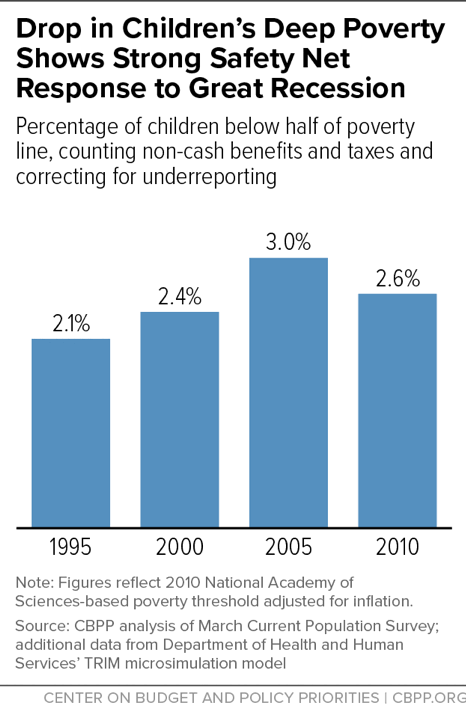
From 2005 to 2010, by contrast, the children’s deep poverty rate fell from 3.0 percent to 2.6 percent after correcting for underreporting.[54] (See Figure 10.) The decline, occurring despite the Great Recession, shows the striking effectiveness of economic security programs during this period, when policymakers supplemented programs’ built-in responsiveness through recovery policies such as expansions in tax credits and temporary measures such as an increase in SNAP benefit levels and enactment of the Making Work Pay tax credit.[55]
Appendix
Changes in CBO’s Methodology
CBO’s methodology for analyzing the distribution of household income and taxes changed little between 2001 and 2012. CBO’s primary measure to rank households and calculate average federal tax rates was a broad measure of “before-tax income” that included both “market income”[56] and a broad set of government transfers. The latter included both social insurance benefits (Social Security, Medicare, unemployment insurance, and workers’ compensation) and means-tested transfers, both cash and in-kind, such as Medicaid and Children’s Health Insurance Program benefits, SNAP benefits, and TANF cash assistance.[57] “After-tax income” equaled this “before-tax income” minus federal individual and corporate income, payroll (social insurance), and excise taxes.
In its 2012 distributional analysis covering the years 1979-2009, CBO made two significant changes to its methodology for computing income, one concerning who bears the burden of corporate income taxation and the other concerning how CBO values government-provided health insurance such as Medicare and Medicaid.[58] CBO also made the consequential decision to switch from a version of the consumer price index (CPI) to the personal consumption expenditure (PCE) price index in calculating real income (i.e., income after adjusting for inflation). The PCE index generally shows lower inflation than the CPI and hence faster real income growth.
In previous reports, CBO had assumed that that the entire burden of corporate income taxes fell on owners of capital, so it subtracted 100 percent of corporate tax payments from the income of owners of capital in calculating after-tax income. Based on a review and analysis of the economic literature, CBO changed to allocating 25 percent of the corporate tax burden to workers and the remaining 75 percent to owners of capital.
CBO’s previous method for measuring the value of government-provided health insurance aimed to measure the extent to which this coverage frees up income that a household can then use to meet basic food or housing expenses. That method capped the value of government-provided health insurance that is counted as income at the smaller of the actual cost to the government of providing the insurance and the maximum amount the household could afford to pay for health insurance without compromising its ability to meet other basic needs. The revised method that CBO put in place in 2012 uses the government’s average cost of providing health insurance to the household (as CBO has long done in valuing employer-provided health insurance benefits). For many low-income households, however, this approach produces a significantly higher measured income, while leaving the amount of cash income actually available to meet other basic needs unchanged.[59]
In 2018, CBO made another substantial change, switching to use of “income before transfers and taxes” to rank households and calculate effective tax rates. Broadly speaking, this new measure consists of market income plus social insurance benefits, such as Social Security and Medicare. More specifically, it includes all cash income (including non-taxable income not reported on tax returns, such as child support), taxes paid by businesses,[60] employees’ contributions to 401(k) retirement plans, and the estimated value of in-kind income such as Medicare and employer-paid health insurance premiums. One effect of this change appears to be to shift more seniors with substantial Medicaid benefits — which, as a means tested entitlement, aren’t counted as income under this measure — into the bottom fifth of the income distribution.[61]
As part of this 2018 revision, CBO also created its second new measure, “income after transfers and taxes.” It consists of the former “after-tax income” plus means-tested transfers, such as Medicaid and SNAP.[62]
CBO states that the former method of using after-tax income for ranking was appropriate for analyzing the effects of federal taxes, but with the growing importance of means-tested transfers, the change allows the agency to analyze both means-tested transfers and taxes on the same basis. Together with the 2012 change in the treatment of government-provided health insurance, however, this change appears to strongly affect income trends for the poorest households, substantially raising the level and rate of growth of their measured income.
End Notes
[1] See http://www.census.gov/topics/income-poverty/income.html.
[2] Internal Revenue Service, “SOI Tax Stats — Individual Income Tax Returns Publication 1304,” multiple years available, https://www.irs.gov/uac/soi-tax-stats-individual-income-tax-returns-publication-1304-complete-report.
[3] Jesse Bricker et al., “Changes in U.S. Family Finances from 2013 to 2016: Evidence from the Survey of Consumer Finances,” Federal Reserve Bulletin, Vol. 103, No. 3, September 2017, https://www.federalreserve.gov/publications/files/scf17.pdf.
[4] Congressional Budget Office, “The Distribution of Household Income, 2016,” July 9, 2019, https://www.cbo.gov/publication/55413.
[5] Emmanuel Saez, “Striking it Richer: The Evolution of Top Incomes in the United States,” University of California, updated March 2, 2019, https://eml.berkeley.edu/~saez/saez-UStopincomes-2017.pdf.
[6] See Emmanuel Saez and Gabriel Zucman, “Wealth Inequality in the United States Since 1913: Evidence from Capitalized Income Tax Data,” Quarterly Journal of Economics, Vol. 131, No. 2, May 2016, http://eml.berkeley.edu/~saez/SaezZucman2016QJE.pdf; Thomas Piketty, Emmanuel Saez, and Gabriel Zucman, “Distributional National Accounts: Methods and Estimates for the United States,” Quarterly Journal of Economics, Vol. 133, No. 2, May 2018, http://gabriel-zucman.eu/files/PSZ2018QJE.pdf; and Emmanuel Saez and Gabriel Zucman, The Triumph of Injustice: How the Rich Dodge Taxes and How to Make Them Pay, W.W. Norton and Company, 2019.
For a discussion of distributional analyses and frameworks currently in use, see Kevin Perese, “CBO’s New Framework for Analyzing the Effects of Means-Tested Transfers and Federal Taxes on the Distribution of Household Income,” Congressional Budget Office, December 2017, pp. 41-45, https://www.cbo.gov/system/files/115th-congress-2017-2018/workingpaper/53345-workingpaper.pdf.
[7] For 2018, approximately 94,600 housing units were in the sample for the ASEC. About 81,900 housing units were determined eligible for interview and about 68,300 interviews were conducted. Census Bureau, “Source and Accuracy of Estimates for Income and Poverty in the United States: 2018 and Health Insurance Coverage in the United States: 2018,” p. 3, https://www2.census.gov/library/publications/2019/demo/iphi-sa.pdf.
[8] Census also collects data on income, poverty, and health insurance coverage through the American Community Survey (ACS), which has replaced the long-form decennial census questionnaire. For its more limited set of categories, the ACS provides better data at the state and local levels than the CPS, but Census advises that the CPS data provide the best annual estimates of income, poverty, and health insurance coverage for the nation as a whole.
[9] The March supplement to the CPS was expanded to include interviews from February and April and renamed the ASEC in 2001.
[10] Examples of money income — sometimes referred to as “cash income” — include: wages and salaries; income from dividends; earnings from self-employment; rental income; child support and alimony payments; Social Security, disability, and unemployment benefits; cash welfare assistance; and pensions and other retirement income. Census money income does not include non-cash benefits such as those from SNAP, Medicare, Medicaid, or employer-provided health insurance.
[11] Census uses a three-parameter scale for equivalence adjustment that takes into account family size and composition. For example, a two-adult, one-child family has a different adjustment than a one-adult, two-child family.
[12] This is generally referred to as “top-coding” and is done to preserve confidentiality. In addition, in the public-use data files of the ASEC made available to researchers, Census takes further steps to preserve confidentiality for high-income individuals well below this limit by exchanging income values between individuals with very similar values in a procedure called “rank-proximity swapping.”
[13] Internal Revenue Service, “Individual Income Tax Returns 2017,” Publication 1304, Table C, September 2019, https://www.irs.gov/pub/irs-pdf/p1304.pdf.
[14] For the most recent estimates, see Congressional Budget Office (2019), op. cit.
[15] Households with negative income are excluded from the lowest income category but are included in the totals.
[16] Changes in the nature of health care spending also could affect measured income differently than they affect household well-being. For example, advances in medical technology could enhance the value to households of health care spending in ways that the income data would not fully capture. Conversely, spending increases on wasteful medical procedures or larger profit margins in the medical, insurance, or prescription drug industries could result in increases in health care spending that CBO counts as added income but do not enhance recipients’ well-being. A recent paper estimated that waste in the U.S. health care system accounted for approximately 25 percent of health care spending. William H. Shrank, Teresa L. Rogstad, and Natasha Parekh, “ Waste in the US Health Care System: Estimated Costs and Potential for Savings,” JAMA, October 7, 2019, https://jamanetwork.com/journals/jama/fullarticle/2752664.
[17] For details on their methods, see Thomas Piketty and Emmanuel Saez, “Income Inequality in the United States: 1913-1998,” Quarterly Journal of Economics, February 2003, or, for a less technical summary, see Saez’s latest update: “Striking It Richer: The Evolution of Top Incomes in the United States,” March 2, 2019, https://eml.berkeley.edu/~saez/saez-UStopincomes-2017.pdf. Their most recent estimates are available at https://eml.berkeley.edu/~saez/TabFig2018prel.xls.
[18] Piketty and Saez make available three different data series, each of which treats capital gains slightly differently and therefore yields somewhat different estimates of the share of income going to each group. (For example, estimates of the share of income going to the top 1 percent in 2018 vary from 18.46 percent in one series to 20.37 percent in a second series to 21.76 percent in the series we rely on here.) We follow the income concept in Saez’s most recent report and focus on the series that includes capital gains income both in ranking households and in measuring the income that households receive.
[19] More technically, Piketty and Saez calculate market income by taking the adjusted gross income reported on tax returns and then adding back all adjustments to gross income (such as deductions for health savings accounts, student loan interest, self-employment tax, and IRAs). Note that this definition of market income is not the same as the “market income” concept used in the recent CBO report described above.
[20] People with income below certain thresholds are not required to file personal income tax returns. Thresholds are determined according to age and filing status. For example, for 2018 returns filed in 2019, the filing thresholds were $24,000 for a non-elderly married couple and $13,600 for an elderly single person. Many people who are not required to file tax returns nonetheless pay considerable federal taxes, such as payroll and excise taxes, as well as state and local taxes.
[21] They estimate the total number of potential filers from Census data by summing the total of married men, widowed or divorced men and women, and single men and women over age 20. The number of non-filing tax units in their analysis is the difference between their estimated total and the number of returns actually reported in the IRS data. This methodology assumes the number of married women filing separately is negligible, and it has been quite small since 1948. Before that, however, married couples with two earners had an incentive to file separately, and Piketty and Saez adjust their data to account for that.
[22] For the years since 1943, non-filers, who account for a small percentage of all filers and of total income, are assigned an income equal to 20 percent of the average income of filers (except in 1944-45, when the percentage is 50 percent). For earlier years, when the percentage of non-filers and their share of income were much higher, Piketty and Saez assume, based on the ratio in subsequent years, that total market income of filers plus non-filers is equal to 80 percent of total personal income (less transfers) reported in the National Income and Product Accounts for 1929-1943 and as estimated by the economist Simon Kuznets for 1913-1928. For those years, the total income of non-filers is the difference between estimated total income and income reported on tax returns.
[23] According to data from the Bureau of Economic Analysis, wages and salaries now provide about 81 percent of employee compensation; supplemental benefits such as contributions to health and retirement plans provide the rest. In 1980, 85 percent of compensation came through wages and 15 percent through benefits; in 1950, 93 percent came through wages and 7 percent through benefits.
[24] For example, employer-sponsored health insurance benefits likely constitute a much smaller fraction of income for the top 1 percent than for the vast majority of middle-income tax units; their omission could understate income growth in the middle of the distribution relative to growth at the top.
[25] See Piketty, Saez, and Zucman, op. cit.
[26] They provide an alternative analysis in which the earnings of the members of a married couple are assigned to each member individually in order to examine gender inequality.
[27] Many of these choices are inherently arbitrary. In the case of spending on public goods like national defense, for example, how to assign benefits to individual households is more a philosophical question than one that can be resolved analytically or empirically. Piketty, Saez, and Zucman’s decision to use split-income couples in their base case (as opposed to, say, family size-adjusted measures, as CBO does) removes the effect of changes in family size on trends in inequality.
[28] Between 2014 and 2018, Census implemented improvements to the CPS ASEC, introducing new income questions and an updated data processing system to improve income reporting, increase response rates, and reduce reporting errors. In its historical tables, Census reports one set of statistics for 2013 based on the legacy questionnaire and another based on the redesigned questionnaire. Similarly, Census reports one set of statistics for 2017 produced under the old processing system and one produced under the updated system. Census advises caution in comparing estimates from 2018 forward with estimates from before 2017.
[29] When income increases by 100 percent, it doubles. When it increases by 300 percent, it quadruples.
[30] Congressional Budget Office, “Projected Changes in the Distribution of Household Income, 2016-2021,” December 2019, Figure 4, p. 15, https://www.cbo.gov/publication/55941.
[31] This discussion uses the Piketty-Saez estimates based on their analysis of IRS data alone. However, their more ambitious analysis of the distribution of all of national income shows a similar pattern of concentration at the top.
[32] In the Piketty-Saez data, average incomes in 2018 were about $1.5 million for the top 1 percent of households and about $2.3 million for the top 0.5 percent.
[33] Assets include such things as savings, stocks, vehicles, homes, and business and financial assets. Liabilities include such things as credit card debt, mortgages, and past-due bills.
[34] Bricker et al. (2017), op. cit.
[35] Ibid., “Box 3: Recent Trends in Income and Wealth.”
[36] Michael Batty et al., “The Distributional Financial Accounts,” FEDS Notes, August 30, 2019, https://www.federalreserve.gov/econres/notes/feds-notes/the-distributional-financial-accounts-20190830.htm.
[37] Because the two datasets underlying the distributional national accounts use somewhat different wealth concepts and are presented and measured at different frequencies (every three years versus quarterly), the precise changes in the share of different wealth groups over time in the SCF and the distributional national accounts are similar but not identical.
[38] Saez and Zucman (2016), op. cit.
[39] A recent Federal Reserve analysis tries to reconcile differences between the SCF and Zucman-Saez findings through measures such as including estimates for the wealth of the Forbes 400 in the SCF and adjusting upward the assumed rate of return on fixed-income assets held by those at the top in Zucman-Saez. The Fed researchers are able to narrow the gap between the two estimates of top-income shares, and they conclude that their estimates “concur that inequality, at least as reflected in top income and wealth shares, has been rising in recent decades.” See Jesse Bricker et al., “The Increase in Wealth Concentration, 1989-2013,” Federal Reserve Board, June 2015, http://www.federalreserve.gov/econresdata/notes/feds-notes/2015/increase-in-wealth-concentration-1989-2013-20150605.html.
[40] There are 48 official poverty thresholds. These thresholds reflect an equivalence adjustment, but not the same three-parameter scale that Census uses when it equivalence-adjusts household income. CBO uses another equivalence adjustment, based on the square root of the number of household members.
[41] Constance Citro and Robert Michael, eds., Measuring Poverty: A New Approach, Committee on National Statistics, National Research Council, 1995, http://www.nap.edu/openbook.php?isbn=0309051282.
[42] Census publishes eight experimental NAS-based poverty rates in addition to the official poverty rate, each calculated using a slightly different methodology. Estimates of these alternative poverty rates are available for each year from 1999 through 2017. The latest tables are available at https://www.census.gov/data/tables/2017/demo/supplemental-poverty-measure/nas-2017.html. These NAS measures also use a three-parameter equivalence scale to adjust for family size and composition. The NAS report recommended against treating the value of medical benefits as income in measuring poverty, noting ways in which medical benefits do not serve the same role as cash. Instead, the report recommended subtracting out-of-pocket medical expenditures from income, since money spent on medical needs is not available to meet the basic needs of food, clothing, shelter, and utilities upon which the NAS poverty threshold is based.
[43] For more detail, see Liana Fox, “The Supplemental Poverty Measure: 2018,” U.S. Census Bureau, October 2019, https://www.census.gov/content/dam/Census/library/publications/2019/demo/p60-268.pdf.
[44] WIC — the Special Supplemental Nutrition Program for Women, Infants, and Children — provides nutritious food, counseling on healthy eating, and health care referrals to low-income pregnant and postpartum women, infants, and children under age 5 who are at nutritional risk.
[45] Christopher Wimer et al., “Trends in Poverty with an Anchored Supplemental Poverty Measure,” Columbia Population Research Center, December 2013, http://cupop.columbia.edu/publications/2013.
[46] Danilo Trisi and Matt Saenz, “Economic Security Programs Cut Poverty Nearly in Half Over Last 50 Years,” Center on Budget and Policy Priorities, updated November 26, 2019, https://www.cbpp.org/research/poverty-and-inequality/economic-security-programs-cut-poverty-nearly-in-half-over-last-50.
[47] In 2018 Census released data based on an updated processing system. To facilitate comparisons across time, Census released two versions of 2016 and 2017 data: one comparable to 2018, the other comparable to earlier years.
[48] Using data comparable back to the 1960s, the poverty rate stood at a record low of 14.4 percent in 2017, not statistically different from 2000’s 14.6 percent. In 2018, the poverty rate stood at 12.8 percent, using the data released under the new methodology. The Census Bureau also released a 2017 poverty rate that is recalculated using the new methodology so that it is comparable to the 2018 figure; this recomputed 2017 figure is 13.5 percent.
[49] Ibid.
[50] Center on Budget and Policy Priorities, “Chart Book: Economic Security and Health Insurance Programs Reduce Poverty and Provide Access to Needed Care,” updated December 11, 2019, https://www.cbpp.org/research/poverty-and-inequality/chart-book-economic-security-and-health-insurance-programs-reduce.
[51] For more detail, see Arloc Sherman and Danilo Trisi, “Deep Poverty Among Children Worsened in Welfare Law’s First Decade,” Center on Budget and Policy Priorities, July 23, 2014, https://www.cbpp.org/files/7-23-14pov2.pdf and Arloc Sherman and Danilo Trisi, “Safety Net for Poorest Weakened After Welfare Law But Regained Strength in Great Recession, at Least Temporarily,” Center on Budget and Policy Priorities, May 11, 2015, https://www.cbpp.org/sites/default/files/atoms/files/5-11-15pov.pdf.
[52] CBPP corrects for undercounting using data from the TRIM microsimulation model, a policy simulation tool developed and maintained by the Urban Institute for the U.S. Department of Health and Human Services Office of the Assistant Secretary for Planning and Evaluation. TRIM starts with person-by-person Census data from the CPS and adjusts it to better match true numbers of recipients of assistance from program records.
[53] Ife Floyd, Ashley Burnside, and Liz Schott, “TANF Reaching Few Poor Families,” Center on Budget and Policy Priorities, updated November 28, 2018, https://www.cbpp.org/research/family-income-support/tanf-continues-to-weaken-as-a-safety-net.
[54] CBPP analysis finds that corrections for underreporting have a particularly large effect on the poverty-reduction estimates for SNAP. SNAP lifted 10 million people above the SPM poverty line in 2012 with corrections, compared with 5 million people without these corrections. See Arloc Sherman and Danilo Trisi, “Safety Net More Effective Against Poverty Than Previously Thought,” Center on Budget and Policy Priorities, May 6, 2015, https://www.cbpp.org/research/poverty-and-inequality/safety-net-more-effective-against-poverty-than-previously-thought.
[55] Arloc Sherman, “Poverty and Financial Distress Would Have Been Substantially Worse in 2010 Without Government Action, New Census Data Show,” Center on Budget and Policy Priorities, November 7, 2011, www.cbpp.org/cms/?fa=view&id=3610.
[56] “Market income” is labor income (wages, salaries, benefits, and the employer’s share of payroll taxes), business income (net income from business and farms owned solely by their owners, partnership income, and income from S corporations), realized capital gains, other capital income (dividends, rental income, and imputed corporate income taxes), income received in retirement for past services, and income from other sources. Note that this definition of “market income” differs from the market income concept used in the Piketty-Saez analysis discussed in this paper (see footnote 19).
[57] See definitions of social insurance benefits and means-tested programs in CBO (2019), p. 2.
[58] See Congressional Budget Office, “The Distribution of Household Income and Federal Taxes, 2008 and 2009,” July 2012, https://www.cbo.gov/sites/default/files/112th-congress-2011-2012/reports/43373-averagetaxratesscreen.pdf.
[59] Prior to 2012, CBO valued government-provided health insurance on the basis of the Census Bureau’s “fungible value” estimates, which essentially cap the value at the amount that a household could afford to pay for insurance. (Specifically, the cap is set at the amount by which the household’s income exceeds what it needs to meet basic food and housing expenses.) See CBO 2012, op. cit.
For low-income households, the fungible value of government-provided health insurance can be substantially less than the average cost to the government of providing it. Consider a household with $5,500 in income above what it needs to meet basic food and housing expenses. If government-provided health insurance for this type of household costs an average of $10,000, CBO would value the benefit at the full $10,000 under its current approach but at $5,500 under the prior approach, since that is all that the household could afford to spend on insurance in the absence of government-provided insurance. See the supplemental data accompanying Congressional Budget Office, “The Distribution of Household Income, 2016,” July 9, 2019, https://www.cbo.gov/publication/55413.
[60] CBO’s estimates of household income before transfers and taxes include the imputed value of taxes paid by businesses because CBO assumes that businesses would pay equivalently higher wages in the absence of those taxes.
[61] As CBO’s July 2012 report explains (p.18): “[T]he higher valuation of government provided health insurance causes about one-eighth of the households in the bottom quintile under CBO’s earlier methodology (roughly 3 million households) to be classified in the second quintile under CBO’s new methodology, and it causes a corresponding number of households to be classified in the bottom quintile rather than the second quintile. The households who moved out of the bottom quintile generally had much lower cash income than did those who moved into it.”
[62] CBO does not subtract other federal taxes (such as estate and gift taxes) or state and local taxes when calculating income after transfers and taxes. Also, it should be noted that for some low-income households, CBO’s estimated income after transfers and taxes is higher than their estimated income before transfers and taxes due to refundable tax credits.
Más de los autores

Areas of Expertise

Areas of Expertise